Pulsar Timing with HENDRICS, Stingray, and PINT

Contact: youlituo-at-gmail.com

This tutorial shows how to build a synthetic pulsar timing experiment using three tools that are common in high-energy timing analyses:

• Stingray provides data structures and utilities for working with event lists and pulse profiles.

• HENDRICS adds convenient wrappers for folding and extracting times of arrival (TOAs).

• PINT evaluates a timing model against those TOAs and produces timing residuals.

We will simulate photon event times for a slowly spinning down pulsar, recover a set of TOAs from the event data, and compare timing residuals for models with and without a frequency derivative.

Prerequisites

This notebook assumes you are running Python ≥ 3.8 in a clean environment (e.g. a conda env) and have the following packages installed:

# timing tools
pip install stingray hendrics pint-pulsar tat-pulsar

Note

• HENDRICS will pull in a compatible version of Stingray, but for this tutorial we assume a reasonably recent Stingray release (≥ 2.2).

• tat-pulsar is optional and only used in a few convenience functions; you can comment those parts out if you prefer not to install it.

Preparing the data

To process real-life datasets, you need to download the datasets from the archive, possibly run the L2 pipeline, and barycenter correct them with barycorr.

Download

Use the example scripts to browse the HEASARCH through TAP services:

$ wget -q -nH -r -l0 -c -N -np -R 'index*' -erobots=off --retr-symlinks --cut-dirs=5 https://heasarc.gsfc.nasa.gov//FTP/ixpe/data/obs/02/02004001/

Barycentric Correction

Understanding the Barycentric Correction

Precise pulsar timing requires that all photon arrival times be measured in a common inertial reference frame. IXPE records event times in the spacecraft frame, and the spacecraft orbits the Earth, which orbits the Sun. This motion introduces a varying geometric light-travel delay that must be removed before we can search for or model pulsations.

1. Why barycentric correction is necessary

A pulsar emits pulses at extremely stable intervals in its own rest frame.
However, as the Earth (and the spacecraft) move around the Sun, we are sometimes closer to the pulsar and sometimes farther away. This produces a geometric delay known as the Roemer delay.

In the diagram below:

• The dashed line indicates the fixed direction to the pulsar.

• When the Earth is on the near side of its orbit, photons travel a shorter path → the pulses arrive earlier (maximum advance).

• When the Earth is on the far side, the path is longer → the pulses arrive later (maximum delay).

This modulation has an amplitude of up to
\( \pm 500\ \mathrm{s} \times \cos\beta \),
where \( \beta \) is the ecliptic latitude of the source.

For a pulsar with a spin period of order 1 second (like Her X-1), the uncorrected arrival times could shift by hundreds of pulses over the course of the observation.

Barycentric Correction for IXPE

IXPE often distributes more than one orbit file for a given observation. They need to get listed in a text file, and this text file has to be passed with an @ in front when given to barycorr.

$ ls ls -1 hk/ixpe02004001_*orb* > orbit_files
$ barycorr event_l2/ixpe02004001_det1_evt2_v01.fits.gz ixpe02004001_det1_evt2_v01_bary.fits orbitfiles=@orbit_files ra=254.45754588609 dec=35.34235737652 refframe=ICRS ephem=JPLEPH.430

Click to expand output

**** Running barycorr v2.17 ****
: WARNING - input file is .gz gzipped - this may cause problems, especially for large files.
: WARNING - it is recommended to unzip before running this task.
barycorr: shell ftcopy infile='event_l2/ixpe02004001_det1_evt2_v01.fits.gz' outfile='ixpe02004001_det1_evt2_v01_bary.fitsworkfile49668' copyall=YES clobber=YES chatter=0 history=NO
barycorr: running hdaxbary -i '@orbit_files' -f ixpe02004001_det1_evt2_v01_bary.fitsworkfile49668 -jpleph 430 -ra 254.45754588609 -dec 35.34235737652 -ref ICRS
barycorr: shell hdaxbary -i '@orbit_files' -f ixpe02004001_det1_evt2_v01_bary.fitsworkfile49668 -jpleph 430 -ra 254.45754588609 -dec 35.34235737652 -ref ICRS 2>&1
<=== Finished after 3 HDUs
hdaxbary: Using JPL Planetary Ephemeris DE-430
hdaxbary: Using JPL Planetary Ephemeris DE-430
hdaxbary: Using JPL Planetary Ephemeris DE-430barycorr: exited with status 0
barycorr: shell ftchecksum infile='ixpe02004001_det1_evt2_v01_bary.fitsworkfile49668' update=yes datasum=YES chatter=0
barycorr: shell ftcopy infile='ixpe02004001_det1_evt2_v01_bary.fitsworkfile49668' outfile='ixpe02004001_det1_evt2_v01_bary.fits' copyall=YES clobber=YES chatter=0 history=NO
barycorr: barycorr successfully completed

Do the same for all three event lists.

$ barycorr event_l2/ixpe02004001_det1_evt2_v01.fits.gz ixpe02004001_det1_evt2_v01_bary.fits orbitfiles=@orbit_files ra=254.45754588609 dec=35.34235737652 refframe=ICRS ephem=JPLEPH.430
$ barycorr event_l2/ixpe02004001_det2_evt2_v01.fits.gz ixpe02004001_det2_evt2_v01_bary.fits orbitfiles=@orbit_files ra=254.45754588609 dec=35.34235737652 refframe=ICRS ephem=JPLEPH.430
$ barycorr event_l2/ixpe02004001_det3_evt2_v01.fits.gz ixpe02004001_det3_evt2_v01_bary.fits orbitfiles=@orbit_files ra=254.45754588609 dec=35.34235737652 refframe=ICRS ephem=JPLEPH.430

Source Filtering

Use your favorite tool to create a region file and filter the source events from the background. I use ds9 for the region and fselect for event selection

 $ for ev in ixpe02004001_det*v01_bary.fits; do fselect $ev ${ev/.fits/_filt.fits} "regfilter('ds9.reg')" clobber=yes; done

and also select the event files for background region

$ for ev in ixpe02004001_det*v01_bary.fits; do fselect $ev ${ev/.fits/_bkg.fits} "regfilter('back.reg')" clobber=yes; done

!ls -tr 02004001/*fits

02004001/ixpe02004001_det1_evt2_v01_bary_bkg.fits
02004001/ixpe02004001_det1_evt2_v01_bary_filt.fits
02004001/ixpe02004001_det1_evt2_v01_bary.fits
02004001/ixpe02004001_det2_evt2_v01_bary_bkg.fits
02004001/ixpe02004001_det2_evt2_v01_bary_filt.fits
02004001/ixpe02004001_det2_evt2_v01_bary.fits
02004001/ixpe02004001_det3_evt2_v01_bary_bkg.fits
02004001/ixpe02004001_det3_evt2_v01_bary_filt.fits
02004001/ixpe02004001_det3_evt2_v01_bary.fits

Analysis

from stingray import EventList


events1 = EventList.read("02004001/ixpe02004001_det1_evt2_v01_bary_filt.fits", fmt='hea')
events2 = EventList.read("02004001/ixpe02004001_det2_evt2_v01_bary_filt.fits", fmt="hea")
events3 = EventList.read("02004001/ixpe02004001_det3_evt2_v01_bary_filt.fits", fmt="hea")

We can create a single event list from the three. Stingray’s time series classes (EvenList, Lightcurve, etc.) have the join method that can be used to merge together the time series.

events = events1.join(events2)
events = events.join(events3)

/Users/honghui/anaconda/anaconda3/lib/python3.12/site-packages/stingray/base.py:2024: UserWarning: Attribute nphot is different in the time series being merged.
  warnings.warn(

import matplotlib.pyplot as plt
import matplotlib as mpl
mpl.rcParams['figure.dpi'] = 150


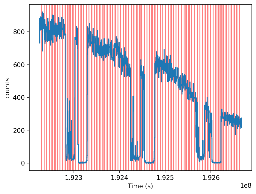
lc = events.to_lc(dt=100)

# This is just to clean up the light curve from all points outside the GTIs, for plotting purposes.
lc.apply_gtis(inplace=True)
lc.plot()

<Axes: xlabel='Time (s)', ylabel='counts'>

Binary-Orbit Correction

After applying the barycentric correction, the photon arrival times are already referenced to the Solar System Barycentre (SSB). However, for binary pulsars like Her X-1, the neutron star is itself orbiting its companion. This motion adds an additional delay that must be removed before we search for or model the spin period.

1. Why binary correction is needed

In a binary system, the pulsar moves around the system’s center of mass.
As it moves:

• When the pulsar is closer to us (approaching), the light-travel time is shorter → pulses arrive earlier.

• When the pulsar is farther (receding), the travel time is longer → pulses arrive later.

This additional delay is called the Roemer delay of the binary orbit.

For Her X-1 (https://gammaray.nsstc.nasa.gov/gbm/science/pulsars/lightcurves/herx1.html):

• Orbital period
  \( P_b \approx 1.7001674\ \text{days} \)

• Projected semi-major axis
  \( x = a_1 \sin i / c = 13.185\ \text{light-seconds} \)

• Eccentricity
  \( e \approx 0 \) (nearly circular)

• Long-term period derivative
  \( \dot{P}_b = -4.93 \times 10^{-11}\ \text{days/day} \)

Because the orbit is nearly circular, the timing modulation is very close to a clean sinusoid with amplitude ~13 seconds. If this effect is not removed, the pulsar phases drift rapidly and the 1.24-second pulse signal becomes smeared over the orbit.

2. What the binary correction computes

For each photon, we compute the difference between the emission time at the pulsar and the arrival time at the SSB:

\[ \Delta t_{\mathrm{bin}}(t) = \frac{a_1 \sin i}{c} \sin \left( \frac{2\pi}{P_b}(t - T_0) \right), \]

in the circular orbit approximation.

In the general case (including eccentricity, periastron advance, or Einstein/Shapiro delays), the full binary model solves Kepler’s equation and evaluates the full BT/ELL1 timing delay. The function tatpulsar.pulse.binarycor.Cor() implements this general binary delay model.

from tatpulsar.pulse.binarycor import Cor
from tatpulsar.utils.functions import met2mjd, mjd2met
import numpy as np

pb = 1.7001674 * 86400 
pb_dot = -4.93e-11
x  = 13.185            # a1 * sin i / c = 1 light-second
e  = 0.0           # eccentricity
t0 = 2449420.67347 - 2400000.5           # periastron time
omega = 0.0        # rad

tw = t0 - 1.7001674/4

t_corr = np.empty_like(events.time)
for i in range(len(events.time)):
    t_corr[i] = Cor(met2mjd(events.time[i], 'ixpe'),
                    tw, e, pb, pb_dot, omega, 0, x, 0)
t_em = events.time + t_corr

/Users/honghui/anaconda/anaconda3/lib/python3.12/site-packages/numba/core/decorators.py:246: RuntimeWarning: nopython is set for njit and is ignored
  warnings.warn('nopython is set for njit and is ignored', RuntimeWarning)

Pulsation search

Once we have barycentric- and binary-corrected event times, the main goal of timing analysis is to detect and measure periodic signals from the pulsar. A pulsation search asks:

“Is there a coherent periodicity in these photon arrival times, and if so, at what frequency (or period)?”

There are several families of tests for this, such as Fourier power spectra, epoch-folding statistics, and phase-based tests. One very widely used phase-based test in high-energy astronomy is the Z-squared (Z²) statistic (Buccheri et al. 1983).

The Z-squared statistic

The Z-squared test works directly on the phases of the photons at a trial signal frequency. For each trial frequency ( \(\nu\) ), we compute the phase of each photon:

\[ \phi_j = \nu t_j \quad (\mathrm{mod}\ 1), \]

where ( \(t_j\) ) is the (corrected) arrival time of photon ( \(j\) ). If there is no pulsation at that frequency, the phases ( \(\phi_j\) ) should be uniformly distributed in ([0, 1)). If a pulsation is present, the phases will tend to cluster, and this can be detected through sinusoidal moments.

For ( \(N\) ) photons and a chosen number of harmonics ( \(n\) ), the ( \(Z_n^2\) ) statistic is defined as

\[ Z_n^2 = \frac{2}{N} \sum_{k=1}^{n} \left[ \left(\sum_{j=1}^{N} \cos k\phi_j \right)^2 + \left(\sum_{j=1}^{N} \sin k\phi_j \right)^2 \right]. \]

• ( N ) is the number of photons.

• ( n ) is the number of harmonics included in the test
  (e.g. (n = 1) for a nearly sinusoidal pulse profile, higher (n) for more complex profiles).

• ( \(\phi_j\) ) are the phases of the events at the trial frequency.

If the phases are purely random (no pulsation), ( \(Z_n^2\) ) follows a chi-square distribution with ( \(2n\) ) degrees of freedom. A strong periodic signal produces a large excess in ( \(Z_n^2\) ) at the true spin frequency (and often at its harmonics).

In Stingray, the Z-squared search is implemented in stingray.pulse.search.z_n_search, which scans a frequency grid and computes ( \(Z_n^2\) ) at each trial frequency.

import numpy as np
from stingray.pulse.search import epoch_folding_search, z_n_search

period = 1/0.807947352321026
nbin = 32
obs_length = events.time.max() - events.time.min()
df_min = 1/obs_length
oversampling = 35
df = df_min / oversampling
frequencies = np.arange(1/period - 200 * df, 1/period + 200 * df, df)

nharm = 2
freq, zstat = z_n_search(t_em, frequencies, nbin=nbin, nharm=nharm)

RuntimeWarning: This platform does not support extended precision floating-point, and PINT will run at reduced precision.

# ---- PLOTTING --------
plt.figure()
plt.plot(freq, (zstat - nharm), label='$Z_2$ statistics')

plt.axvline(1/period, color='r', lw=3, alpha=0.5, label='Correct frequency')
plt.xlim([frequencies[0], frequencies[-1]])
plt.xlabel('Frequency (Hz)')
plt.ylabel('Statistics - d.o.f.')
plt.legend()

<matplotlib.legend.Legend at 0x31738ea50>

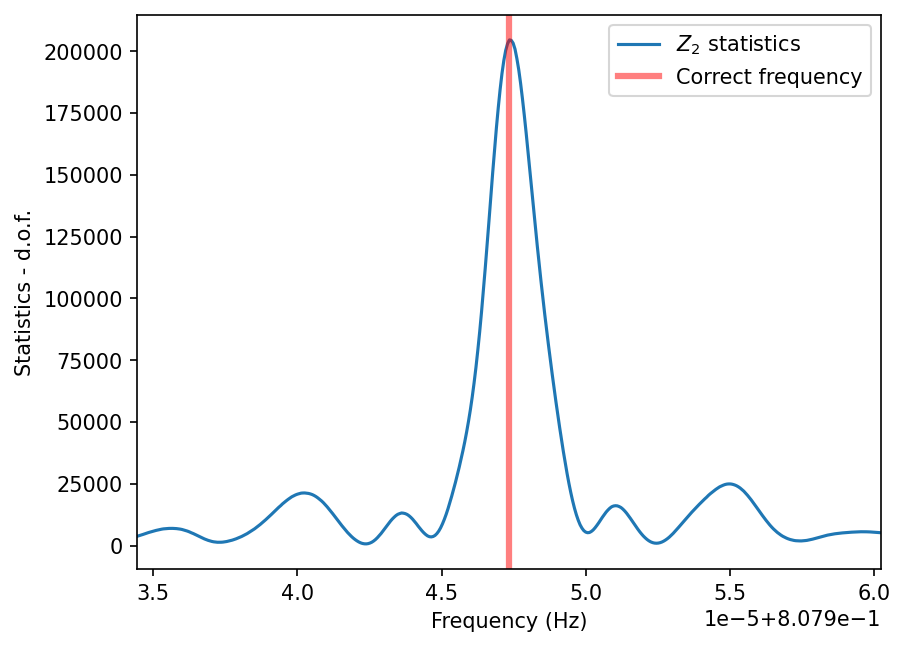
period_best = 1/freq[np.argmax(zstat)]

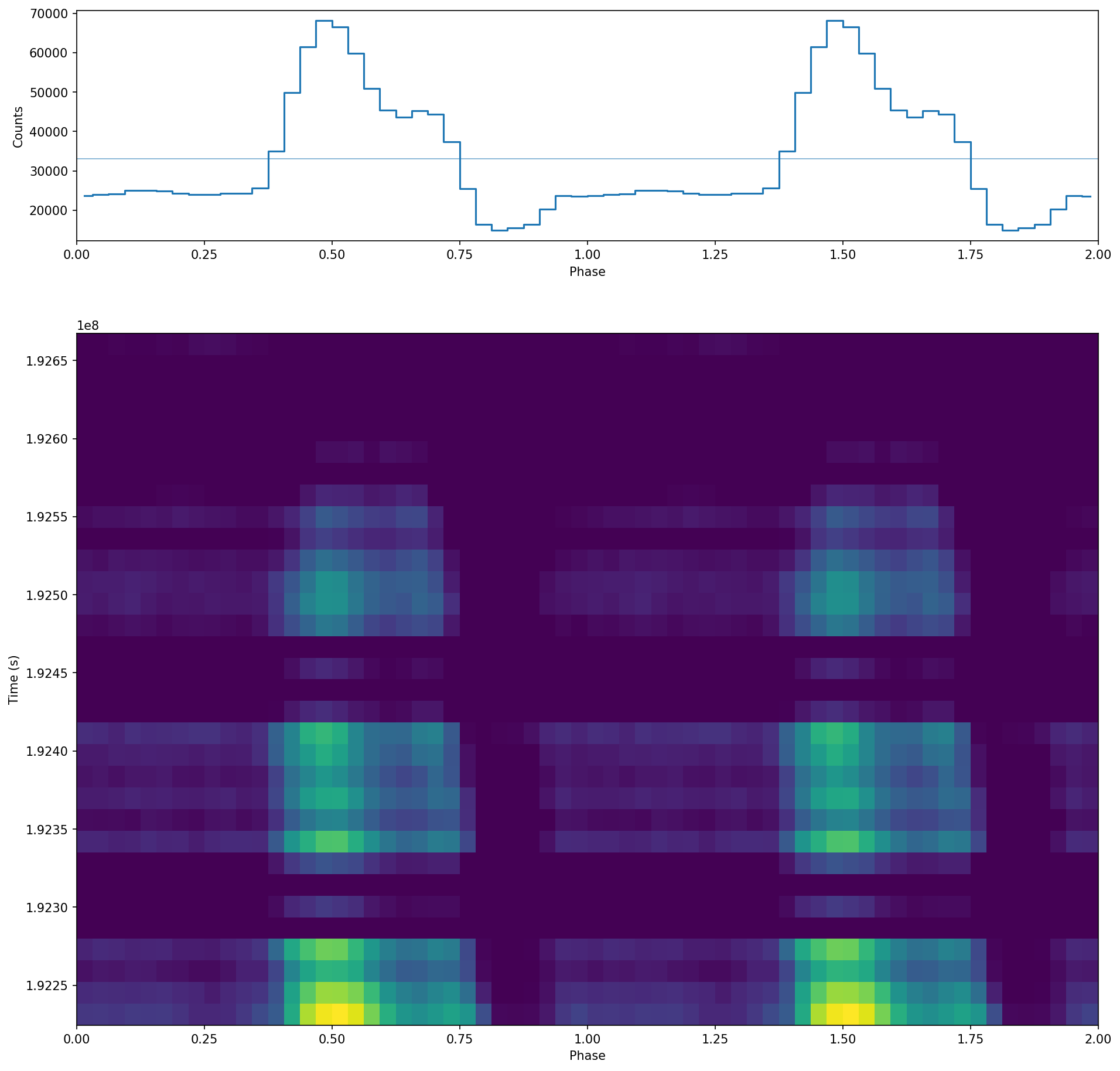
from stingray.pulse.search import phaseogram, plot_phaseogram, plot_profile
from matplotlib.gridspec import GridSpec

# Calculate the phaseogram
phaseogr, phases, times, additional_info = \
            phaseogram(t_em, 1/period_best, return_plot=True, nph=nbin, nt=32)

# ---- PLOTTING --------

# Plot on a grid
plt.figure(figsize=(15, 15))
gs = GridSpec(2, 1, height_ratios=(1, 3))
ax0 = plt.subplot(gs[0])
ax1 = plt.subplot(gs[1], sharex=ax0)

mean_phases = (phases[:-1] + phases[1:]) / 2
plot_profile(mean_phases, np.sum(phaseogr, axis=1), ax=ax0)
# Note that we can pass arguments to plt.pcolormesh, in this case vmin
_ = plot_phaseogram(phaseogr, phases, times, ax=ax1, vmin=np.median(phaseogr))

Pulsar Search with HENDRICS

Read the event time using HENreadevents

$ HENreadevents ixpe02004001_det1_evt2_v01_bary_filt.fits

and after this command a picked file is generated name ixpe02004001_det1_evt2_v01_bary_filt_ixpe_du1_ev.p (ending could be .p or `.nc’ depending on different factors.

$ HENphaseogram -f 0.80794755 ixpe02004001_det1_evt2_v01_bary_filt_ixpe_du1_ev.p -n 64 --norm to1 --pepoch 59981.38359501043 --binary 

adjust the value of those binary parameter to ensure those white lines which predict the modulation of the model to mimic the modulation of the evolution pulse profile

Wooohooo!