HEASOFT, CALDB and NuSTAR data reduction

contact: menglei.zhou@astro.uni-tuebingen.de

0. Prerequisites

0.1. Installation of HEAsoft

excute wget https://heasarc.gsfc.nasa.gov/FTP/software/lheasoft/lheasoft6.36/heasoft-6.36src.tar.gz in your preferred installation directory

and follow the installation guidance at https://heasarc.gsfc.nasa.gov/docs/software/lheasoft/linux.html. It shall take a few hours to finish.

We strongly recommend you to compile the source code to proceed (in order to use local models)!

0.2. Installing the calibration database ($CALDB)

1. follow the guidance at https://heasarc.gsfc.nasa.gov/docs/heasarc/caldb/caldb_install.html to install the calibration database software.

2. cd $CALDB

3. find the calibration files of NuSTAR mission at https://heasarc.gsfc.nasa.gov/docs/heasarc/caldb/caldb_supported_missions.html

4. run wget https://heasarc.gsfc.nasa.gov/FTP/caldb/data/nustar/fpm/goodfiles_nustar_fpm_20251027.tar.gz to download the NuSTAR calibration files.

5. tar -zxf goodfiles_nustar_fpm_20251027.tar.gz

6. for future practice, you may also download the calibration files:

   NICER: wget https://heasarc.gsfc.nasa.gov/FTP/caldb/data/nicer/xti/goodfiles_nicer_xti_20240206.tar.gz;

   IXPE: wget https://heasarc.gsfc.nasa.gov/FTP/caldb/data/ixpe/gpd/goodfiles_ixpe_gpd_20250225.tar.gz & wget https://heasarc.gsfc.nasa.gov/FTP/caldb/data/ixpe/xrt/goodfiles_ixpe_xrt_20241028.tar.gz

   and unzip them in $CALDB. The calibration files will be delivered to the proper position automatically.

0.3. Installing DS9 (for image handling)

go to https://sites.google.com/cfa.harvard.edu/saoimageds9 and follow the installation guidance

1. Accessing Observational Data from High-Energy Astrophysics Archives

go to https://heasarc.gsfc.nasa.gov/cgi-bin/W3Browse/w3browse.pl and search for your interested source

e.g., the famous galactic black hole binary: Cygnus X-1

1.1. Download the level 1 data (the preprocessed data of your observation)

wget -q -nH --no-check-certificate --cut-dirs=6 -r -w1 -l0 -c -N -np -R 'index*' -erobots=off --retr-symlinks https://heasarc.gsfc.nasa.gov/FTP/nustar/data/obs/10/9//91002320002/

2. Run the pipeline to produce the NuSTAR level 2 data (clean photon event lists)

nupipeline indir=/data/to/your/path/91002320002 outdir=/data/to/your/path/91002320002/out steminputs=nu91002320002

This step is quite time-consuming and may take several hours to complete. But don’t worry — we’ve already prepared the processed results for you! You can download them here: https://drive.google.com/file/d/1MqZozxRo7Rp7XxY6zoU5GqNI5Fz_Volm/view?usp=sharing

2.1. The FITS file structure (HDU := Header + Data)

2.2. Header

2.3. Data

3. Using DS9 to extract the source region and the background region

ds9 out/nu91002320002A01_cl.evt and ds9 out/nu91002320002B01_cl.evt

Please refer to https://heasarc.gsfc.nasa.gov/docs/nustar/analysis/nustar_quickstart_guide.pdf as a quick-start guide and https://heasarc.gsfc.nasa.gov/docs/nustar/analysis/nustar_swguide.pdf for further details.

In brief, the source region should encompass most of the emission area when viewed on a logarithmic color scale, while the background region should be as large as possible—excluding any part of the source—and selected from the same detector quadrant.

4. Extract the spectra and light curves (level 3 data that can be used directly for scientific purposes.)

nuproducts srcregionfile=./out/src.reg bkgregionfile=./out/bkg.reg indir=./out outdir=./products instrument=FPMA steminputs=nu91002320002 bkgextract=yes

nuproducts srcregionfile=./out/src.reg bkgregionfile=./out/bkg.reg indir=./out outdir=./products instrument=FPMB steminputs=nu91002320002 bkgextract=yes

the whole process can take 10+ minutes to complete. Or you can get the products via https://drive.google.com/file/d/1vXcH7zNuNQT6ojTcW6iQM6l2KcuxV5FZ/view?usp=sharing

5. Check the structure of your final scientific products

We can use fv to quickly check the structure of FITS files. fv NAME_OF_YOUR_INTERESTED_FILE.fits (.evt .lc .pha .rmf .arf ...)

5.1. The structure of light curve files

the correlation between rate_orginal and rate:

5.2. The structure of the spectrum

Next, we’ll handle more complex FITS files—most of these operations can be done conveniently with astropy.

import numpy as np
import astropy.io.fits as fits
import matplotlib.pyplot as plt

5.2.1. Spectrum file

spec = fits.open('../data/nu91002320002A01_sr.pha')
spec.info()

Filename: ../data/nu91002320002A01_sr.pha
No.    Name      Ver    Type      Cards   Dimensions   Format
  0  PRIMARY       1 PrimaryHDU     504   (105, 105)   float32   
  1  SPECTRUM      1 BinTableHDU    468   4096R x 2C   [J, J]   
  2  GTI           1 BinTableHDU     57   13R x 2C   [1D, 1D]   
  3  REG00101      1 BinTableHDU     84   1R x 6C   [1PD(1), 1PD(1), 16A, 1PD(1), 1PD(0), 1PI(1)]   

bkg_spec = fits.open('../data/nu91002320002A01_bk.pha')
bkg_spec.info()

Filename: ../data/nu91002320002A01_bk.pha
No.    Name      Ver    Type      Cards   Dimensions   Format
  0  PRIMARY       1 PrimaryHDU     504   (143, 143)   float32   
  1  SPECTRUM      1 BinTableHDU    468   4096R x 2C   [J, J]   
  2  GTI           1 BinTableHDU     57   13R x 2C   [1D, 1D]   
  3  REG00101      1 BinTableHDU     84   1R x 6C   [1PD(1), 1PD(1), 16A, 1PD(1), 1PD(0), 1PI(1)]   

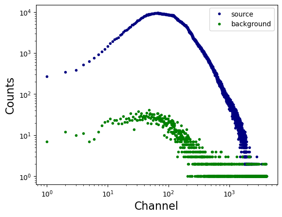
x = spec['SPECTRUM'].data['CHANNEL']
y = spec['SPECTRUM'].data['COUNTS']

plt.loglog(x, y, linestyle = 'none', marker = '.', markerfacecolor = 'navy', markeredgecolor = 'navy', label = 'source')

x = bkg_spec['SPECTRUM'].data['CHANNEL']
y = bkg_spec['SPECTRUM'].data['COUNTS']

plt.loglog(x, y, linestyle = 'none', marker = '.', markerfacecolor = 'green', markeredgecolor = 'green', label = 'background')

plt.xlabel('Channel', fontsize = 16)
plt.ylabel('Counts', fontsize = 16)

plt.legend()
plt.show()

5.2.2. Response Matrix Files (RMFs)

resp = fits.open('../data/nu91002320002A01_sr.rmf')
resp.info()

Filename: ../data/nu91002320002A01_sr.rmf
No.    Name      Ver    Type      Cards   Dimensions   Format
  0  PRIMARY       1 PrimaryHDU      14   ()      
  1  EBOUNDS       1 BinTableHDU     58   4096R x 3C   [J, E, E]   
  2  MATRIX        1 BinTableHDU     52   4096R x 6C   [E, E, I, PI(117), PI(117), PE(4027)]   

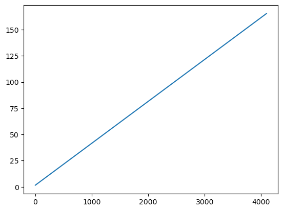
plt.plot(resp['EBOUNDS'].data['CHANNEL'], resp['EBOUNDS'].data['E_MIN'])
plt.show()

print(resp['EBOUNDS'].data['E_MAX'] - resp['EBOUNDS'].data['E_MIN'])

[0.03999996 0.03999996 0.04000008 ... 0.03999329 0.03999329 0.04000854]

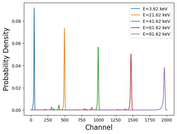
x = resp['EBOUNDS'].data['CHANNEL']

idx_1 = 50
idx_2 = 500
idx_3 = 1000
idx_4 = 1500
idx_5 = 2000

y = resp['MATRIX'].data['MATRIX'][idx_1]/np.sum(resp['MATRIX'].data['MATRIX'][idx_1])
plt.plot(y, label = 'E={0:0.2f} keV'.format(resp['EBOUNDS'].data['E_MIN'][idx_1] + 0.02))

y = resp['MATRIX'].data['MATRIX'][idx_2]/np.sum(resp['MATRIX'].data['MATRIX'][idx_2])
plt.plot(y, label = 'E={0:0.2f} keV'.format(resp['EBOUNDS'].data['E_MIN'][idx_2] + 0.02))

y = resp['MATRIX'].data['MATRIX'][idx_3]/np.sum(resp['MATRIX'].data['MATRIX'][idx_3])
plt.plot(y, label = 'E={0:0.2f} keV'.format(resp['EBOUNDS'].data['E_MIN'][idx_3] + 0.02))

y = resp['MATRIX'].data['MATRIX'][idx_4]/np.sum(resp['MATRIX'].data['MATRIX'][idx_4])
plt.plot(y, label = 'E={0:0.2f} keV'.format(resp['EBOUNDS'].data['E_MIN'][idx_4] + 0.02))

y = resp['MATRIX'].data['MATRIX'][idx_5]/np.sum(resp['MATRIX'].data['MATRIX'][idx_5])
plt.plot(y, label = 'E={0:0.2f} keV'.format(resp['EBOUNDS'].data['E_MIN'][idx_5] + 0.02))

plt.legend()

# plt.yscale('log')

plt.xlabel('Channel', fontsize = 16)
plt.ylabel('Probability Density', fontsize =16)

plt.show()

5.2.3. Ancillary Response Files (ARFs)

arf = fits.open('../data/nu91002320002A01_sr.arf')
arf.info()

Filename: ../data/nu91002320002A01_sr.arf
No.    Name      Ver    Type      Cards   Dimensions   Format
  0  PRIMARY       1 PrimaryHDU      12   ()      
  1  SPECRESP      1 BinTableHDU     88   4096R x 3C   [E, E, E]   

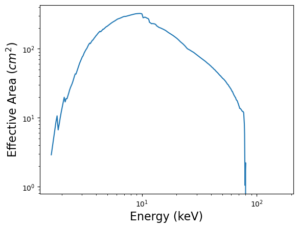
x = 0.5*(arf['SPECRESP'].data['ENERG_LO'] + arf['SPECRESP'].data['ENERG_HI'])
y = arf['SPECRESP'].data['SPECRESP']

plt.loglog(x, y)
plt.xlabel('Energy (keV)', fontsize = 16)
plt.ylabel('Effective Area ($cm^2$)', fontsize = 16)

plt.show()

5.3. Group your spectra so that Gaussian statistics can be validly applied

ftgrouppha nu91002320002A01_sr.pha nu91002320002A01_sr_grp.pha grouptype=optmin groupscale=30 respfile=nu91002320002A01_sr.rmf clobber=yes

ftgrouppha nu91002320002B01_sr.pha nu91002320002B01_sr_grp.pha grouptype=optmin groupscale=30 respfile=nu91002320002B01_sr.rmf clobber=yes

please read https://heasarc.gsfc.nasa.gov/docs/software/lheasoft/help/ftgrouppha.html for further details.

6. Fit your spectra with XSPEC

Simply enter xspec in the command prompt to start XSPEC.

We often adopt the elemental abundances of the Galaxy as defined by the solar abundances measured by Wilms et al. (2000). To set this in XSPEC, type abund wilm in the XSPEC prompt.

Type query yes to prevent the program from requesting further confirmations until you obtain the best fit.

6.1. Loading the data into XSPEC

data 1:1 nu91002320002A01_sr_grp.pha

data 2:2 nu91002320002B01_sr_grp.pha

(The number before the colon specifies how many model sets you want to fit, while the number after the colon indicates the spectrum number. Try running data 1:1 nu91002320002A01_sr_grp.pha and data 1:2 nu91002320002B01_sr_grp.pha, then define a model to observe the difference.)

ignore 1-2: **-3.0 79.0-** (This command excludes the poorly calibrated energy ranges. Note: Always include the decimal point — otherwise, XSPEC will interpret the value as a channel number instead of an energy value.)

6.2. Fitting

The model is calculated in flux space and then transformed into channel space using the response matrix and the effective area.

• C(I): the expectation of the observed count spectrum;

• S(E): the (defined) intrinsic source spectrum (in flux space);

• R(I, E): the normalized instrumental response matrix;

• A(E): the effective area of the instrument;

• B(I): the background spectrum.

Type model constant*TBabs*powerlaw in XSPEC.

constant — accounts for the flux normalization between the two NuSTAR instruments, FPMA and FPMB.

TBabs — represents Galactic absorption.

powerlaw — describes the spectral continuum, which is primarily dominated by inverse Compton scattering.

Simply type fit once all parameters have been set.

cpd /xs or cpd /xw to set the proper plotting window

plot uf del: this is the command to show the unfolded spectrum (in flux space) and the \(\chi\) residuals.

We can see a very porminent iron line and some humps at 20-30 keV.

Or we can try model constant*TBabs*(powerlaw + diskbb) to consider the contribution from the accretion disk.

The iron line is still there, not resolved by the thermal disk model diskbb.

Or we can try model constant*TBabs*(powerlaw + diskbb + gaussian) to cover the Gaussian line at 6-7 keV.

What should be the best model? We can try with some physical models…

constant*TBabs*(nthcomp + relxill + gaussian), how about this?

The details of the relxill model family will be discussed in the following lectures!