Timing Analysis#
contact: menglei.zhou@astro.uni-tuebingen.de
0. Prerequisites#
Installation Stingray package using pip or conda
Note that our recommendation to use Stingray is not because it is indispensable for timing analysis, but simply because it is Python-based and easy to work with. In fact, you can always write your own code if you prefer.
1. Extract a light curve (with Energy filtered) from an event list#
def gti_extraction(gti_info):
    gti_str = "["
    gti_sum = 0.0
    for gti_element in gti_info:
        gti_str = gti_str + "[{0:0.1f}, {1:0.1f}], ".format(gti_element[0], gti_element[1])
        gti_sum += gti_element[1] - gti_element[0]
    gti_str = gti_str[:-2] + "]"
    return gti_str, gti_sum
import os
import numpy as np
import matplotlib.pyplot as plt
import astropy.io.fits as fits
from stingray import Lightcurve, Powerspectrum, AveragedPowerspectrum, Crossspectrum, AveragedCrossspectrum
# Some basic FITS file reading work...

evt_file = fits.open('ni2596010601_0mpu7_cl.evt')
evt_file.info()
Filename: ni2596010601_0mpu7_cl.evt
No.    Name      Ver    Type      Cards   Dimensions   Format
  0  PRIMARY       1 PrimaryHDU      32   ()
  1  EVENTS        1 BinTableHDU    289   504165R x 14C   [1D, 1B, 1B, 1I, 1I, 1B, 1B, 8X, 1K, I, J, 1I, 1I, 1E]
  2  FPM_SEL       1 BinTableHDU    122   3387R x 3C   [1D, 56B, 56I]
  3  GTI           1 BinTableHDU    254   2R x 2C   [D, D]
  4  GTI_MPU0      1 BinTableHDU    253   2R x 2C   [D, D]
  5  GTI_MPU1      1 BinTableHDU    253   2R x 2C   [D, D]
  6  GTI_MPU2      1 BinTableHDU    253   2R x 2C   [D, D]
  7  GTI_MPU3      1 BinTableHDU    253   2R x 2C   [D, D]
  8  GTI_MPU4      1 BinTableHDU    253   2R x 2C   [D, D]
  9  GTI_MPU5      1 BinTableHDU    253   2R x 2C   [D, D]
 10  GTI_MPU6      1 BinTableHDU    253   2R x 2C   [D, D]
# Select the photons within 0.4 - 10 keV range
# Recall that for NICER, PI ~ 100*Energy (keV)

idx = np.greater_equal(evt_file['EVENTS'].data['PI'], 40) & np.less_equal(evt_file['EVENTS'].data['PI'], 1000)
print(idx)
print(len(evt_file['EVENTS'].data[idx]))
[ True  True  True ...  True  True  True]
500828
When creating a light curve from an event list, always remember to explicitly set the GTI, T_start, and T_stop. This is essential—otherwise your products may show incorrect count rates, or you may not be able to ensure that light curves from different energy bands are strictly simultaneous.
photon_event_time = evt_file['EVENTS'].data['TIME'][idx]
delta_t = 0.001953125
gti, gti_len = gti_extraction(evt_file['GTI'].data)

t_start = evt_file['GTI'].data[0][0]
t_stop = evt_file['GTI'].data[-1][1]

lc = Lightcurve.make_lightcurve(photon_event_time, dt = delta_t, gti = eval(gti), tstart = t_start, tseg = t_stop - t_start)
print(lc)
Lightcurve
__________
time           : [1.66323159e+08 ... 1.66330209e+08] (size 3609600)
time (MJD)     : [1925.03656251 ... 1925.11815971]
counts         : [0 ... 0] (size 3609600)
dt             : 0.001953125
err_dist       : poisson
high_precision : False
input_counts   : True
low_memory     : False
mjdref         : 0
notes          :
tseg           : 7050.0
tseg (MJD)     : 0.08159722222222222
tstart         : 166323159.0
tstart (MJD)   : 1925.0365625
gti            : [[1.66323159e+08 1.66324638e+08]
 [1.66328690e+08 1.66330209e+08]] (shape (2, 2))
gti (MJD)      : [[1925.0365625  1925.05368056]
 [1925.1005787  1925.11815972]]
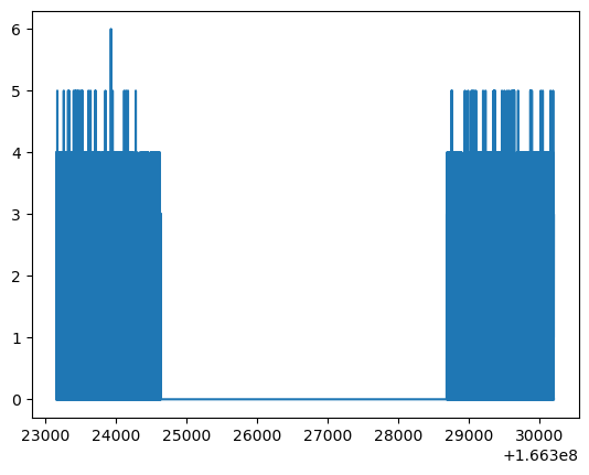
plt.plot(lc.time, lc.counts)
plt.show()
2. Some basic knowledge on Fourier Transform#
Better refer to Wikipedia: Discrete Fourier Transform, van der Klis (1988), or the PhD thesis of Katja Pottschmidt (2002).
In brief: we have a light curve \(x(t) = [x(t_0), x(t_1), x(t_2), x(t_3), \dots, x(t_{N-1})]\), the discrete Fourier transform (DFT) can be computed with
where \(x_k\) denotes the \((k+1)\)-th component \(x(t_k)\).
The corresponding Fourier frequencies are given by
The flux decomposition as a function of frequency can be expressed as
which defines the inverse discrete Fourier transform (IDFT).
We notice that \(\exp\left( \frac{2 \pi {\bf i} j k}{N} \right) = \exp\left[ - \frac{2 \pi {\bf i} \left( N - j \right) k}{N} \right]\), which implies that frequencies corresponding to indices \(j > N/2\) are typically considered negative frequencies. Since each pair of positive and negative frequencies results in DFT components that are complex conjugates when \(x_k\) is real, we discard the negative frequencies and focus solely on the positive ones.

Practically, we prefer to set \(N\) as a power of 2 to enable the Fast Fourier Transform (FFT). In this case, \(N\) is even. The minimum nonzero frequency is given by \(f_\text{min} = 1/T = 1/(N \Delta t)\), while the highest physical frequency, known as the Nyquist frequency, is \(f_\text{max} = 1/(2\Delta t)\).
3. Produce the power spectrum from a light curve#
The power spectral density (PSD) is a real quantity to represent the squared magnitude of the complex products of DFT of a time series:
The uncertainties of the PSD are on the same order of magnitude as the PSD values themselves. However, these uncertainties can be reduced by averaging over more samples (as the mean value of the power scales with \(1/\sqrt{N}\), in which \(N\) is the sample number). We can average the PSDs not only across multiple segments of a long light curve but also within different frequency bins to reduce the uncertainties of the PSD.
Three commonly-seen norms in the power spectrum:
where \(R\) is the mean count rate and \(T\) denotes the length of the segment.
Q: Why the normalization of power spectrum matters?
A: The expected power and Poisson noise levels differ under each normalization. For convenience, we often choose different normalizations for different tasks—for example, comparing power spectra between two sources or subtracting white noise.
Leahy normalization and fractional rms normalization each offer distinct advantages. Leahy normalization allows for straightforward estimation and subtraction of Poisson noise. In contrast, fractional rms normalization makes the power spectral densities (PSDs) independent of the source’s mean count rate, enabling direct comparison of timing properties across sources with different luminosities, masses, or spectral states.
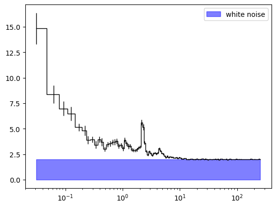
ps = AveragedPowerspectrum.from_lightcurve(lc, 16384*delta_t, norm = 'leahy')
ps_rebin = ps.rebin_log(f = 0.05)
print(ps_rebin)
0it [00:00, ?it/s]
93it [00:00, 8784.18it/s]
AveragedPowerspectrum
_____________________
freq           : [3.1250000e-02 ... 2.5390625e+02] (size 124)
k              : [  1 ... 133] (size 124)
m              : [   93 ... 12369] (size 124)
power          : [14.83058  ...  1.986109] (size 124)
power_err      : [1.53785951 ... 0.01795936] (size 124)
unnorm_power   : [39659.28322723 ...  5311.16511857] (size 124)
unnorm_power_err: [4112.47609543 ...   48.02613017] (size 124)
df             : 0.03125
dt             : 0.001953125
err_dist       : poisson
gti            : [[1.66323159e+08 1.66324638e+08]
 [1.66328690e+08 1.66330209e+08]] (shape (2, 2))
mean           : 0.32643504809307794
n              : 16384
norm           : leahy
nphots         : 5348.311827956989
nphots1        : 5348.311827956989
save_all       : False
segment_size   : 32.0
show_progress  : True
type           : powerspectrum
plt.errorbar(ps_rebin.freq, ps_rebin.power, yerr = ps_rebin.power_err, ds = 'steps-mid', \
             color = 'black', linewidth = 1.0)
plt.fill_between(ps_rebin.freq, 0.0, 2.0, color = 'blue', alpha = 0.5, label = 'white noise')
plt.xscale('log')
plt.legend()
# plt.yscale('log')
plt.show()
3.1. Fit the power spectrum in XSPEC#
We first prepare a power spectral data file in a specific format to emulate an actual spectrum file.
Then, we create an identity matrix to serve as the response matrix for the power spectrum.
The spectral file should follow the format:
energy_lo energy_hi photon_flux photon_flux_err
and use the tool ftflx2xsp to create those PHA/RMF files.
For more details, please refer to the documentation at: https://heasarc.gsfc.nasa.gov/docs/software/lheasoft/help/ftflx2xsp.html
psd_spectrum_filename = 'psd.dat'
psd_pha_file = 'psd.pha'
psd_rsp_file = 'psd.rsp'

f = ps_rebin.freq
power_sig = ps_rebin.power - 2.0
power_err = ps_rebin.power_err

with open(psd_spectrum_filename, 'w') as file:
    for i in range(len(f)):
        if i == 0:
            delta_f = 0.5*(f[i+1] + f[i]) - (2.0*f[i] - 0.5*(f[i+1] + f[i]))
            file.write('{0:0.8e} {1:0.8e} {2:0.8e} {3:0.8e}\n'.format(2.0*f[i] - 0.5*(f[i+1] + f[i]), 0.5*(f[i+1] + f[i]), power_sig[i]*delta_f, power_err[i]*delta_f))
        elif i == len(f) - 1:
            delta_f = 2*f[i] - 0.5*(f[i] + f[i-1]) - 0.5*(f[i] + f[i-1])
            file.write('{0:0.8e} {1:0.8e} {2:0.8e} {3:0.8e}\n'.format(0.5*(f[i] + f[i-1]), 2*f[i] - 0.5*(f[i] + f[i-1]), power_sig[i]*delta_f, power_err[i]*delta_f))
        else:
            delta_f = 0.5*(f[i] + f[i+1]) - 0.5*(f[i] + f[i-1])
            file.write('{0:0.8e} {1:0.8e} {2:0.8e} {3:0.8e}\n'.format(0.5*(f[i] + f[i-1]), 0.5*(f[i] + f[i+1]), power_sig[i]*delta_f, power_err[i]*delta_f))
file.close()

cmd_flx2xsp = 'ftflx2xsp {0} {1} {2} clobber=yes'.format(psd_spectrum_filename, psd_pha_file, psd_rsp_file)
print(cmd_flx2xsp)
# os.system(cmd_flx2xsp)
ftflx2xsp psd.dat psd.pha psd.rsp clobber=yes
XSPEC12> data psd.pha
XSPEC12> model lorentz + lorentz + lorentz + lorentz

4. Produce the cross spectrum from two simultaneous light curves#
Let \(x_k\) and \(y_k\) be two light curves with identical time resolution (\(\Delta t\)) and total duration (\(T\)). The cross spectrum between the two light curves is defined as
where \(X_j\) and \(Y_j\) are the DFTs of \(x_k\) and \(y_k\), respectively. Unlike the PSDs, the cross spectrum is generally a complex quantity. When multiple segments of equal length are available, the cross spectrum can be averaged across segments to improve statistical robustness.
# Select the photons within 1 - 5 keV range

idx_1 = np.greater_equal(evt_file['EVENTS'].data['PI'], 100) & np.less_equal(evt_file['EVENTS'].data['PI'], 500)

photon_event_1_5 = evt_file['EVENTS'].data['TIME'][idx_1]
delta_t = 0.001953125

gti, gti_len = gti_extraction(evt_file['GTI'].data)

t_start = evt_file['GTI'].data[0][0]
t_stop = evt_file['GTI'].data[-1][1]

lc_1_5 = Lightcurve.make_lightcurve(photon_event_1_5, dt = delta_t, gti = eval(gti), tstart = t_start, tseg = t_stop - t_start)

# Select the photons within 5 - 10 keV range

idx_2 = np.greater_equal(evt_file['EVENTS'].data['PI'], 500) & np.less_equal(evt_file['EVENTS'].data['PI'], 1000)

photon_event_5_10 = evt_file['EVENTS'].data['TIME'][idx_2]
delta_t = 0.001953125

gti, gti_len = gti_extraction(evt_file['GTI'].data)

t_start = evt_file['GTI'].data[0][0]
t_stop = evt_file['GTI'].data[-1][1]

lc_5_10 = Lightcurve.make_lightcurve(photon_event_5_10, dt = delta_t, gti = eval(gti), tstart = t_start, tseg = t_stop - t_start)
cs = AveragedCrossspectrum.from_lightcurve(lc_1_5, lc_5_10, 16384*delta_t, norm = "leahy")
cs_rebin = cs.rebin_log(f = 0.05)
print(cs_rebin)
0it [00:00, ?it/s]
93it [00:00, 3152.97it/s]
AveragedCrossspectrum
_____________________
freq           : [3.1250000e-02 ... 2.5390625e+02] (size 124)
k              : [  1 ... 133] (size 124)
m              : [   93 ... 12369] (size 124)
power          : [ 4.08998301+0.27585242j ... -0.02845011+0.00788449j] (size 124)
power_err      : [0.61683409+0.44881173j ... 0.01267998+0.01267379j] (size 124)
unnorm_power   : [3966.77614925+267.54262977j ...  -27.59308082  +7.64697243j] (size 124)
unnorm_power_err: [598.25255061+435.29170384j ...  12.29800862 +12.29200114j] (size 124)
channels_overlap: False
countrate1     : 140.2016129032258
countrate2     : 26.208333333333332
df             : 0.03125
dt             : 0.001953125
err_dist       : poisson
fullspec       : False
gti            : [[1.66323159e+08 1.66324638e+08]
 [1.66328690e+08 1.66330209e+08]] (shape (2, 2))
lag_err        : [0.1108364 ... 0.9181087] (size 8191)
mean           : 0.11839306007934904
mean1          : 0.2738312752016129
mean2          : 0.051188151041666664
n              : 16384
norm           : leahy
nph            : 1939.7518963400546
nphots         : 1939.7518963400546
nphots1        : 4486.451612903225
nphots2        : 838.6666666666666
power_type     : all
save_all       : False
segment_size   : 32.0
show_progress  : True
type           : crossspectrum
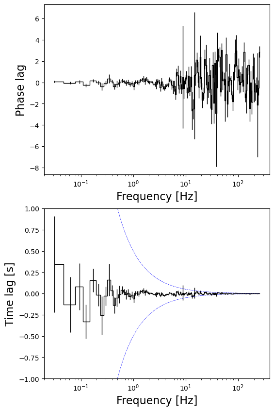
5. Phase lag and Time lag#
In practice, the real and imaginary components of the cross spectrum do not have straightforward physical interpretations on their own. Therefore, any physical conclusions drawn from either component should be made with caution.
However, the phase lag between two light curves can be defined using the argument of the cross spectrum:
This phase lag \(\phi (\nu_j)\) can be related to its corresponding Fourier frequency \(\nu_j\) to yield the time lag:
which represents the time delay, at each frequency band \(\nu_j\), between the two light curves \(x_k\) and \(y_k\).
It is important to note that phase lags are inherently limited to the range \(\left(−\pi, \pi \right]\) due to their periodic nature. Consequently, the corresponding time lags \(\delta t (\nu_j)\) also have a bounded absolute value, especially at low frequencies where small changes in phase can result in large variations in \(\delta t\). As a result, it is not always straightforward to connect measured phase or time lags directly to specific physical processes.
time_lags, time_lags_err = cs_rebin.time_lag()
phase_lags, phase_lags_err = cs_rebin.phase_lag()

# time_lag = phase_lag / (2. * np.pi * freq)
plt.plot(time_lags - phase_lags / (2. * np.pi * cs_rebin.freq))
plt.show()
/Users/honghui/anaconda/anaconda3/lib/python3.12/site-packages/stingray/fourier.py:1134: UserWarning: n_ave is below 30. Please note that the error bars on the quantities derived from the cross spectrum are only reliable for a large number of averaged powers.
  warnings.warn(
fig, axs = plt.subplots(2, 1, figsize=(6,10))
axs[0].errorbar(cs_rebin.freq, phase_lags, yerr = phase_lags_err, ds = 'steps-mid', color = 'black', linewidth = 1.0)
axs[0].set_xscale('log')
axs[0].set_xlabel('Frequency [Hz]', fontsize = 16)
axs[0].set_ylabel('Phase lag', fontsize = 16)

axs[1].errorbar(cs_rebin.freq, time_lags, yerr = time_lags_err, ds = 'steps-mid', color = 'black', linewidth = 1.0)
axs[1].set_xscale('log')
axs[1].set_xlabel('Frequency [Hz]', fontsize = 16)
axs[1].set_ylabel('Time lag [s]', fontsize = 16)

axs[1].plot(cs_rebin.freq, np.pi/(2.0* np.pi * cs_rebin.freq), linestyle = '--', linewidth = 0.5, color = 'blue')
axs[1].plot(cs_rebin.freq, - np.pi/(2.0* np.pi * cs_rebin.freq), linestyle = '--', linewidth = 0.5, color = 'blue')
axs[1].set_ylim((-1, 1))

plt.show()